Finite Element Analysis on Loudspeaker

16th October 2005

This article serve to introduce Finite Element Method to the general public and demonstrate the amount of consideration required when performing a particular task, so that it's importance and care to initiate the method is not neglected.

The following are pieces taken out from my Final Year Project for my B.Eng.(Hons.)Electroacoustics, which is 57 pages, summarized to this page.

The loudspeaker behaviour will be analysed through Finite Element Method with the assistance of ANSYS, a finite element software package. Specific Modal and Harmonic analysis will be carried out under linear conditions without damping effects. The loudspeaker will be analysed in three stages where the first is in vacuum, the second is with a cabinet and finally the last stage takes the acoustic fluid coupling into considerations. The problem will be solved mainly in two-dimension axisymmetric format. Some three-dimensional results will be included to facilitate explanation. Results were obtained to the structural break-up frequencies and shapes, pinpoint structural displacement, vector flow in fluid space, pressure distributions, sound pressure level and others.

The issue of “Damping” is included due to more findings and understanding. A rerun of the Driver’s Modal and Harmonic Analysis is performed and compared against Acoustic Fluid Coupling in each respective analyses section. Note: this is a double extra objective not stated in the project plan.

The loudspeaker (cone in particular) will be analysed under “Finite Element Method”. The FEM idea is to divide the structure into very small pieces, called mesh. The mesh must be smaller than the wavelength under test. This is to allow the assumption that small mesh size will not bend and behaves like a rigid piece. By doing so the complex differential equations will be converted/simplified into linear algebraic matrix set. A computer program called ANSYS/ED version 5.5.1 will solve the huge amount of calculations. The use of FEA enables us to produce information regarding “Cone Break-ups” and it’s “Harmonic content, Sound Radiation Pattern, Sound Pressure Level” and etc.

Finite Element Method (FEM) is a numerical technique capable of analysing any problem within limits. The idea is to split (discretise) the problem domain into small pieces (meshes) called elements so that each can be solved separately, unlike differential equations. The solution is then in the form of a piecewise-smooth function where more elements usually yields better results.

Elements are joint to each other by nodes and care must be exercised to ensure the element edges continue to adjacent elements and do not overlap or separate. It has to satisfy the basic requirement that deformations of a continuous medium must be compatible. This behaviour is controlled by the element shape functions.

The nodes are used as solution points and contain all necessary unknown degrees of freedom (DOF). Since the elements are small as compared to the wavefront of the problem domain, their geometries are simple such as: line, square, triangle or cuboids, therefore linear algebraic equations are used instead of differential equations. It is easier to solve compared to solving the entire structure at once using differential equations. Elements are called “finite” to distinguish them from differential element used in calculus.

All objectives including extras that were stated in the project plan have been achieved. The achieved results are specific to the structure’s break-up (mode) frequencies and shapes, pinpoint structural displacement, vector flow in fluid space, pressure distributions, sound pressure level (SPL) and others. Some results are not true to real world performance due to incompatible damping parameters with ANSYS. Without it all excitation of the loudspeaker will have maximum displacement and not accurate

1.1 skipped

Struck [2] describe Modal Analysis as a process to characterise the dynamic properties of an elastic structure in terms of its modes of vibration.  Vibration energy will cause deformation, known as mode shapes. It occurs at the natural frequency (f_n), each having individual damping. Each mode can then be defined by the f_n, damping factor and mode shape. These parameters can be determined from frequency response measurements at various points.

By comparing a measurement of the driver’s near-field response with a measurement made using an accelerometer mounted on the diaphragm, it is possible to find the frequency (f) above which the driver no longer behaves like a rigid piston.

The two measurements should have the same high-pass characteristic up to this f. Below which the near-field response is proportional to acceleration. This f could also be calculated by finding ka £ 1. For the loudspeaker used in this project a = 0.06545, therefore f = 834Hz. The results shown in Section 4 do not agree with this and an explanation will be given.

By monitoring the current applied to the driver using a small (0.1W) series resistor, the excitation can be calibrated directly in force units (Newton), where F(f) = Bl.i(f) or Bl.[0.1v](f). This is useful because the FE model is excited physically and not electrically, therefore the force used is in Newton. However the actual loudspeaker is not available for testing and hence 1 Newton per node will be used.

Another method of investigating cone behaviour is described in FRANKFORT [3] but it is not using FEM. The differential equations are set up to describe the cone vibration and in the absence of analytical solution, it is solved numerically over a large frequency range. This method is somewhat out-dated (1978) but it explains the cone behaviour very well and is a very interesting loudspeaker reading material.

The second phase is to analyse the effects with an enclosure where Sakai ET AL [4] describe the standing waves in it as being one of the degrading factors and are known to occur at higher frequency range.

Conventional designs use lining and absorptive materials to reduce the standing wave effects. The application of Finite Element to the acoustic cavity has made it possible to discuss a method to reduce inherent standing waves accurately and without needing lining materials.

The paper also describe methods used to obtain enclosure internal radiation impedance, sound pressure distributions and standing waves, where the last is especially investigated through different driver locations, semi apex angles, radius and mass of the driving surface.

ARIE ET AL [5] states in a simplified theory that the radiation impedance of a loudspeaker is often approximated by that of a rigid plane piston in an infinite baffle or at the end of a long tube. However the radiation from a plane piston and that from a non-plane radiator like a loudspeaker are quite different, which is called the cavity effect. To calculate the exact sound radiation from a radiating surface with an arbitrary shape the Helmholtz equation will have to be solved.

However the equation can only be solved analytically for some simple shapes such as a piston in an infinite baffle or a pulsating sphere. For a plane radiator in an infinite baffle the Helmholtz equation reduces to the Rayleigh integral.

For more complicated shapes such as cone or dome loudspeaker the Helmholtz equation has to be solved numerically. This can be done directly using a set of integral equations or with the aid of FEM.

S.-W. Wu ET AL [6] stress to insure the Sommerfield radiation condition at infinity [7, 8] must be enforced, which is no energy may be reflected back to source.

BEM [9, 10, 11] is well suited for external radiation analysis because discretisation of elements is at the model level. It automatically removes the Sommerfield radiation condition problem faced by FEM. No air (fluid) will need to be elementised. It saves a lot of computing power and storage space.

Using FEM for external radiation will be a good hands-on experience to find out the benefit/deficit it gives.

The derivation and proofs, integration points of the FE fundamentals will not be discussed due to overwhelming formulation involved. The following information is provided on a “need to know” basis for the sole purpose of this project. The readers are referred to ANSYS (on-line) Manual [12] (over a thousand pages) specifically the Theory Manual and others, and [13, 14, 15, 16] for further details.

The Structural and Acoustical Fluid Fundamentals will be briefed. Importance is stressed on the Element Shape Functions, Modal Analysis and Harmonic Analysis. Damping will also be briefed.

Stress and strain will not be discussed (21 pages) since the objective of this project is not to analyse the stress and strain of the loudspeaker. Still they are fundamentals and influence the structure behaviour significantly and critical readers are referred to ANSYS Manuals [12] or FE textbooks [13, 14, 15, 16] for further details. Nodal solutions are always provided, but not element solutions. If element solution is turn “ON” then stress and strain will be calculated.

The Structural Matrix used by ANSYS is shown in equation (2.1-1). It represents the equilibrium equation on a one (1) element basis. It is an advanced equation of motion taking a lot of variables into account (i.e. behaviour due to material properties, etc).

                     (2.1-1)

 where: [K_e]      = ò_vol[B]^T[D][B]d(vol)         = element stiffness matrix

            [K_e^f]     = kò_areaf[N_n]^T[N_n]d(areaf)    = element foundation stiffness matrix

            {u}                                                 = nodal displacement vector

            {F_e^th}   = ò_vol [B]^T[D]{e^th}d(vol)     = element thermal load vector

            [M_e]     = rò_vol[N]^T[N]d(vol)           = element mass matrix

            {ü}                                                 = acceleration vector (gravity effects)

            {F_e^pr}   = ò_areap[N_n]^T{p}d(areap)      = element pressure vector

            [F_e^nd]                                              = nodal forces applied to the element

 and to explain the terms contain in “where:”

            vol        = volume of element

            [B]       = strain-displacement matrix, based on element shape functions

            ^T          = current temperature at the point in question

            [D]       = elasticity matrix

            k          = foundation stiffness in units of force per length per unit area

            [N_n]     = matrix of shape functions for normal motions at the surface

            areaf     = area of the distributed resistance

            {e^th}    = thermal strain vector

            r          = density                           

            {p}      = the applied pressure vector

                           (normally contains only one non-zero component)

The Acoustic Governing Equations adopted in the FE matrices derivation process are:

 Acoustic wave equation                                                            (2.2-1)

 Helmholtz equation                                                                       (2.2-2)

 Where the symbols have their usual meanings in acoustics.

The fluid element used in this project will be using equation (2.2.1-1) for analysis.

[M_e^p]{}+[K_e^p]{p_e}+r₀[R_e]^T{U}={0}                                  (2.2.1-1)

where:  [M_e^p]    = 1/c² ò_vol{N}{N}^Td(vol)   = fluid mass matrix (fluid)

            [K_e^p]    = ò_vol­[B]^T[B]d(vol)              = fluid stiffness matrix (fluid)

               r₀[R_e]   = r₀ò_s{N}{n}^T{N’}^Td{s}  = coupling mass matrix (fluid-structure-interface)

Unless forced on, the following damping is ignored as in (2.2.1-1). The infinite acoustic fluid (Fluid129) must take this into account in order to achieve “Minimal reflections” and must use the “DAMPED” analysis method, which forces this term to be included. This is true for Modal Analysis but for Harmonic Analysis it automatically takes damping into account.

[M_e^p]{}+[C_e^p]{}+[K_e^p]{p_e}+r₀[R_e]^T{Ü}={0}                (2.2.2-1)

where:  [C_e^p]  = b/c ò_s{N}{N}^Td(S)   = fluid damping matrix

The interaction of the fluid and structure causes the acoustic pressure to exert a force applied to the structure and the structural motions produce an effective “fluid load”. The governing finite element matrix equations then becomes:

 [M_s]{Ü} + [K_s]{u} = {F_s} + [R]{p}                            (2.2.3-1)

 [M_f]{} + [K_f] {P} = {F_f}-r₀[R]^T{Ü}                        (2.2.3-2)

[R] is the “coupling” matrix that represents the effective surface area associated with each node on the fluid-structure interface (FSI). The coupling matrix [R] also takes into account the direction of the normal vector defined for each pair of coincident fluid and structural element faces that comprises the interface surface. The positive direction of the normal vector, as the ANSYS program uses it, is defined to be outward from the fluid mesh and in towards the structure. Both the structural and fluid load quantities that are produced at the fluid-structure interface are functions of unknown nodal degrees of freedom. Placing these unknown “load” quantities on the left hand side of the equations and combining the two equations into a single equation and adding in the damping term produces the following:

    (2.2.3-3)

where:  [M^fs]  = r₀[R_e]^T

            [K^fs]  = [R_e]

Element Shape Functions are formulas describing the object behaviour under motion, be it excited like loadings or natural frequencies. In short they represent the real object in terms of a huge mathematical expression.

This element is used to model the loudspeaker and cabinet structure.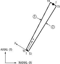

Nodes     = 2 at I and J

DOF       = UX, UY, UZ and ROTZ

It is defined by two nodes, two-end thickness, the number of harmonic waves (MODE), a symmetry condition (ISYM) and the orthotropic material properties.

However isotropic material properties are used because orthotropic material properties are extremely difficult to derive or obtain due to its directional complexity. Orthotropic will be explained in Section 4 – Results and Discussion.

Figure 2.3.1-1 SHELL61 Axisymmetric-Harmonic Structural Shell

Extreme orientations of the conical shell element result in a cylindrical shell element or an annular disc element. Some thick shell effects have been included in the Extra Shape Function (ESF) formulation but it cannot be properly considered to be a thick shell element. If these effects are important, it is recommended to use PLANE25. This element assumes a linear elastic material. This “Thick Shell” problem will be analysed in Section 4 – Results and Discussions.

Axisymmetric Harmonic Shells with ESF

        (2.3.1-1)          (2.3.1-2)(2.3.1-3)

Together they form the stiffness matrix for Shell61. The mass matrix is formed by

                                          (2.3.1-4)

                                          (2.3.1-5)

                  (2.3.1-6)

Axisymmetric Harmonic Shells without ESF

                               (2.3.1-7)

                                (2.3.1-8)

(2.3.1-9)

The pressure load vector is same as the stiffness matrix. This element shape functions is taken from ZIENKIEWICZ [16] by ANSYS.

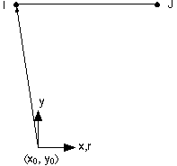
This element is used to model the air (fluid) medium and the interface at fluid-structure-interaction (FSI) problems.

Nodes = 4 at I, J, K, L (or 3 for TRI)

DOF    = UX, UY, UZ and PRES

The translations are applicable only at nodes that are on the interface. This will be a problem when the structural displacement overshoots (infinity) pass into other non-flowing fluid element. This will be seen in a lot of results in Section 4 – Results and Discussion.

Figure 2.3.2-1 FLUID29 2-D Acoustic Fluid

It is defined by four nodes, a reference pressure and the isotropic material properties. The reference pressure (PREF) is used to calculate the element sound pressure level (defaults to 20x10^-6 N/m²). The speed of sound Ö(k/r₀) the fluid is input by SONC where k is the bulk modulus of the fluid (Force/Area) and r_o is the mean fluid density (Mass/Volume) (input as DENS).

FSI may be flagged by surface loads at the element faces as shown by the circled numbers on Figure 2.3.2-1. Specifying the FSI will couple the structural motion and fluid pressure at the interface. The flag specification should be on the fluid elements at the interface.

The element has the capability to include damping of sound absorbing material at the interface. The dissipative effect due to fluid viscosity is neglected, but absorption of sound at the interface is accounted for by generating a damping matrix using the surface area and boundary admittance at the interface.

The acoustic pressure in the fluid medium is determined by the wave equation with the following assumptions:

1.      The fluid is compressible (density changes due to pressure variations).

2.      In-viscid fluid (no dissipative effect due to viscosity).

3.      There is no mean flow of the fluid.

4.      The mean density and pressure are uniform throughout the fluid. Note that the acoustic pressure is the excess pressure from the mean pressure.

5.      Analyses are limited to relatively small acoustic pressures so that the changes in density are small compared with the mean density.

A typical 2D and Axisymmetric 4 node Quadrilateral Solid without ESF (Q4) is used

          (2.3.2-1)

           (2.3.2-2)

The Fluid Stiffness Matrix

      (2.3.2-3)

Together they form the coupled stiffness, mass and fluid damping matrix all taking FSI into account.

This element is used to envelope the model made of FLUID29. FLUID129 realises a second-order absorbing boundary condition so that an outgoing pressure wave reaching the boundary of the model is "absorbed" with minimal reflections back.

Nodes = 2 at I and J

DOF    = officially XTR1 but can be said NONE

It is defined by two nodes (I,J), the material properties and the real constants (RAD). The element must be circular with radius RAD and centre located at or near the centre of the structure. The element is characterized by a pair of symmetric stiffness and damping matrices.

Figure 2.3.3-1 FLUID129 2-D Infinite Acoustic Element

It is recommended that the enclosing circular boundary is placed at a distance of at least 0.2 ´ l from the boundary of any structure that may be submerged in the fluid, where l = c/f is the dominant wavelength of the pressure waves; c is the speed of sound (SONC) in the fluid, and f is the dominant frequency of the pressure wave. For example, in the case of a submerged circular cylindrical shell of diameter D, the radius of the enclosing boundary, RAD, should be at least (D/2) + 0.2 ´ l.

The element formulation can be found in (2.2.1-1).

The modal analysis is used to find the mode shape of the structure at different resonant frequency. It is a quick way to obtain the number of modes within a frequency range. The mode shapes can also be obtained through harmonic analysis by exciting the structure sinusoidally over the desired frequency range by using a small but sufficiently strong signal. However it never produce spot-on resonant frequency because harmonic analysis carries out excitation in steps and may miss the exact frequency. The other down point is too many frequency points are wasted because they are not the resonant frequency.

ANSYS only performs linear analysis unless other features are forced “ON”. The equation of motion for un-damped system, expressed in matrix notation is:

                                                   (2.4-1)

For linear harmonic vibrations 2.4-1 becomes:

                                             (2.4-2)

 But the equality is satisfied if , which is trivial and of no interest therefore 2.4-2 becomes:

                                                        (2.4-3)

The result is provided in the form of natural frequency instead of w.

It uses the subspace iteration technique, which internally uses the generalized Jacobi iteration algorithm. It is highly accurate because it uses the full [K] and [M] matrices.

The Block Lanczos eigenvalue solver uses the Lanczos algorithm where the Lanczos recursion is performed with a block of vectors. This method is as accurate as the subspace method, but faster. The Block Lanczos method uses the sparse matrix solver, overriding any solver specified via the EQSLV command.

It is especially powerful when searching for eigenfrequencies in a given part of the eigenvalue spectrum of a given system. The convergence rate of the eigenfrequencies will be about the same when extracting modes in the midrange and higher end of the spectrum as when extracting the lowest modes.

It is meant for problems where damping cannot be ignored. It uses full matrices ([K], [M], and the damping matrix [C]) and the Lanczos algorithm and calculates complex eigenvalues and eigenvectors (as described below). Sturm sequence checking is not available for this method. Therefore, missed modes are a possibility at the higher end of the frequencies extraction. This is reflected when performing the acoustic coupled modal analysis and will be shown in Section 4 – Results and Discussions and Section 5 – Damping Analysis.

This analysis solves the time-dependent equations of motion for linear structures undergoing steady-state vibration. It will not calculate transient effects. The “Full” matrices solution will be used.

The general equation of motion:

                                    (2.5-1) 

where the symbols have their usual meanings and that {F^a} = applied load vector

Although the entire structure is moving on the same frequency but not necessarily in phase and if damping is included then there is phase shift, therefore the displacements are defined by

                                                        (2.5-2)

where: u_max   = maximum displacement

            j        = imaginary

            W      = imposed circular frequency (radians/time) = 2pf

            f        = imposed f from start to end range

            t        = time     

            f       = displacement phase shift

Note that u_max and f may be different at each DOF therefore 2.5-2 becomes

                                                 (2.5-3)

 where: {u₁} = {u_max cos f} = real displacement vector

            {u₂} = {u_max sin f}   = imaginary displacement vector

The force vector can be specified analogously to the displacement as

                                                (2.5-4)

where: {F₁} = {F_max cos f}    = real force vector

           {F₂} = {F_max sin f} = imaginary force vector

Substituting equation 2.5-3 and 2.5-4 into 2.5-1 becomes

                           (2.5-5) 

The dependence e^jWt is same on both sides and is removed.

The damping matrix [C] may be used in Harmonic, Damped Modal. In its most general form, it is

                       (2.6-1)

where:  [C]          = structure damping matrix

            a             = constant mass matrix multiplier

            [M]         = structure mass matrix

            b             = constant stiffness matrix multiplier

            b_c            = variable stiffness matrix multiplier

            [K]          = structure stiffness matrix

            NMAT    = number of material with DAMPING

            b_j            = constant stiffness matrix multiplier for material j

            [K_j]         = portion of structure stiffness matrix based on material j

            NEL       = number of elements with specified damping

            [C_k]        = element damping matrix

            [C_x]         = frequency-dependent damping matrix

b_c, is used in Harmonic Analysis with Full Frontal Solution. It gives a constant damping ratio regardless of frequency. The damping ratio is actual damping over critical damping.

b_c = x / pf

Damping in some form should be specified other wise the response will be infinity at the resonant frequencies. This will be reflected in a lot of results shown in Section 4 – Results and Discussions. In order to include frequency-dependent damping ratio, the Mass Damping (AlphaD) and Stiffness Damping (BetaD) should be used. Else the Constant Damping Ratio should be used for all frequency range.

The models required for FE analyses are split into three categories due to three different boundary conditions. They are: -

1)      In Vacuum

2)      In Vacuum with Cabinet

3)      Acoustic Fluid Coupling 

A number of macro files are provided in the CD-rom, which performs the modelling, meshing and appropriate analysis. They do not require any action from the user apart from running it in ANSYS. Explanations of how to use the files are contained in Appendix A.

The element discretisation are: -

L1 Coil                = 4 Straight Line

L2 Former           = 6 Straight Line

L3 Cone              = 16 equal length SpLine

L4-15 Surround = 12 Segmented SpLine

Constraint            = 1 at edge of Surround

Excitation            = 5 at Coil 5 nodes

Strength               = 1 Newton each

Direction             = Up along Y-axis

There are 38 structural elements with 39 nodes, each with 4 DOF.

The elements discretisation are: -

L16 Cabinet     = 62 Arc Line

Constraint         = 1 at edge of X-axis

KEYOPT(3)    = 1 (ESF thick shells)

Previous Driver’s constraint is removed.

There are now a total of 100 structural elements

with 101 nodes, each with 4 DOF.

Fluid in contact with the structure.                     Fluid not in contact with the structure.

KEYOPT(2) = 0 = Structure present                KEYOPT(2) = 1 = Structure absent

Both KEYOPT(3) = 1 = axisymmetric. Default is planer, which may be wrong.

Figure 3.3-1  Red = present, Blue = absent       Figure 3.3-2 6171 Elements, 5770 Nodes

Figure 3.3-3                                                     Figure 3.3-4

Mesh L17,18 = 4, L19 = 6, L20,22,24-39,41 = 1, L40 = 62, L42,43 = AUTO, L47 = 3, L48 = 20

10kHz element size èc ¸ 10kHz = 0.0343, then l ¸ 4 minimum criteria = 8.575e-3

L44,46 = 0.57m = l = c ¸ 120Hz (Lf), discretised by 0.57 ¸ 8.57e-3 = 66.47 ~ 67

L45 = inner radius = 0.17m, circumference = 0.534m, then ¸ 8.57e-3 ~ 62

But in order to correlate mesh with Cabinet (covering 150°), then 62 ¸ 5 ´ 6 ~ 74

L43 = outer radius = 0.74m, circumference = 2.325m (left AUTO)

QUAD       = quadrilateral = square shape

TRI            = triangle shape

MAPPED = uniform size

FREE         = free size

1 or 10       = SMARTSIZE (vary 1 to 10)

A1,19        = QUAD,FREE,1

A2             = QUAD,FREE,10

A3,18,20   = QUAD,MAPPED

A4-17        = TRI,FREE,10

A21           = TRI,FREE,1

Figure 3.3-5 Manual meshing    + FSI Flags

After which is Section 4 Results. Since the source for the calculation is from a un-disclosed party, where I agreed not to show, hence no real results will be shown. Below please find some non-directly useful information.

There are three main sections, each analysing a different boundary condition. First is In Vacuum, then In Vacuum with Cabinet and finally with Acoustic Fluid Coupling. All sections include Modal and Harmonic analysis. Damping issue will be a section of its own.

In Vacuum means no frontal and rear acoustic radiation impedance influence from air loading.

ANSYS analysis settings: -

·          Preferences                      = Structural, h-method

·          Analysis Type                  = Modal

·          Analysis Options              = Subspace

·          No. modes to extract       = 100

·          Expand mode shapes        = YES

·          No. modes to expand       = 100

·          Calculate elements results         = YES

·          Start Frequency                = 0Hz

·          End Frequency                 = 10000Hz

This analysis took less than 5 seconds and used 2.3MB for results. It produced 36 modal frequencies from which 10 are in-planes (Z-axis). The In-plane modes correspond to the 3D model rotation behaviour.

Compare 2D_mode_3 = 308.5Hz

(Figure 4.1.1-1) versus 3D_mode_22_&_23 = 309.7Hz

(Figure 4.1.1-2 & 3)

                                                                                                    Figure (4.1.1-1) In-plane mode shape

(Figure 4.1.1-1) shows that the deflection in the planer direction is not a lot. It will correlate to the 3D mode deflection in terms of a small rotation movement as shown in (Figure 4.1.1-2 & 3). 

Figure (4.1.1-2)                                                Figure (4.1.1-3)

This effect is due to symmetrical object have two modes of vibration in the same frequency but at different axis, namely the X&Y-axis FRANKFORT [3].

The 3D model above is too coarse in terms of mesh size and is therefore re-meshed with higher density. This time it produced only one mode at 308Hz unlike the previous 3D pair. The mode shape is shown in (Figure 4.1.1-4). It is still rotating but difficult to be seen. Please see animation 308Hz rotation.avi as provided in the CD-rom using the provided program animate.exe and use the “options” radio button to delay playback speed.

                                                                                      Figure 4.1.1-4

The first natural frequency is 13.7Hz. This is too low for a loudspeaker. It is due to the acquisition of the material properties value not taking the Spider Suspension into account by [1]. The values were manually tuned in conjunction with laser measurements to give highest correlation around the mid frequencies, using 1.5kHz as the reference point. This model will never give good correlation at low frequency or any analytical solution that assumes rigid piston movement.

For example, according to the thiele-small parameters the fs is 43Hz and under vacuum conditions without cabinet it will simply roll off at fs.

When taking cabinet acoustic coupling into account  fc = 95Hz. See Figure (4.1.1-5).

                                                                                                                                                                                                    Figure 4.1.1-5

The Cone’s first mode of vibration starts at 1450Hz (Figure 4.1.1-6) with very minor deflection while the first major deflection is 3800Hz (Figure 4.1.1-7).

The minor deflection may not be said as the Cone’s first real mode because it is extremely close to the Surround where the Surround is deflecting a lot and pulling the Cone out of place. See (Figure 4.1.1-6).

When the break up shape, location and frequency is known an improvement may be applied to the Cone structure to eliminate the break up. One method is to bound strips of other material to the appropriate sections, not forgetting the changes to the new sectional material property values. (Figure 4.1.1-8 & 9) shows how the strips can be applied either to the front of the back or incorporated during manufacturing. It is obvious that this would be more expensive but it is an open option to be considered.

Figure 4.1.1-6                                                  Figure 4.1.1-7

Figure 4.1.1-8                                                  Figure 4.1.1-9

All 36 modes are summarised in (Figure 4.1.1-15) the Cone’s nodal displacement from centre to Surround and (Figure 4.1.1-16) from Cone to edge. One node is shared between the two materials. In this case the stronger element (high stress and strain) dominates, which is the Cone. A summary of the combined Cone and Surround Modal Analysis Nodal Y Displacement is placed in Appendix C.

Figure 4.1.1-15

Figure 4.1.1-16

ANSYS analysis settings: -

·          Preferences                          = Structural, h-method

·          Analysis Type                      = Harmonic

·          Analysis Options                  = Full

·          DOF printout format           = Amplitude + phase

·          Equation solver                    =  everything default

Load Step Options – Time/Frequency – Frequency and Substeps

·          Harmonic Frequency Range  = 0 to 10000

·          No. of Substeps                    = 500

·          KBC                                     = Ramped

This analysis took 3 minutes and used 31MB for results.

(Figure 4.1.2-1) shows the averaged nodal displacement of the Cone and Surround surface. This is to make a direct comparison with the modal frequencies from (4.1.1). There are 22 noticeable peaks with 3800Hz especially high at 1.69e-3. That is the first major mode of vibration from (4.1.1). There is a small ripple just above 3800Hz, which is another mode. 13.7Hz and 197Hz are covered and cannot be seen. There is only 1 mode left unaccounted for. Perhaps the amplitude may be too small to be seen by the naked eye.

Figure 4.1.2-1

This is the most difficult model to perform. The Modal Analysis has to be carried out stage by stage to insure that it is producing reasonable results. First, internal coupling is analysed under “Modal” where it gave some expected results but lack of density (insufficient fluid modes etc). The mesh sizes had to be refined until it could reach 10kHz, but it did not. The maximum obtainable modal frequency is 7284.2Hz. Another model was created which double all elements around 2000 but the frequency dropped to 5000+.

After countless checking, Self-Confidence ruled that it has been modelled correctly and that the 7284.2Hz model is adopted. After adding external coupling it produced a lot of modes as expected (lots of fluid mode) and finally the Infinite Acoustic Element is applied and the analysis results obtained.

If Modal Analysis does not produce good results then Harmonic Analysis cannot be performed.

The following short discussions are based on the model without infinite acoustic element, i.e. not a “Damped” solution but “Unsymmetric”. The output requested is Amplitude and Phase. This is a Modal Analysis with Internal and External Acoustic Coupling.

The output Mode Frequencies are shown in (Table 4.3-1).

      Table 4.3-1

Contour Nodal UY will be showing set 1=13.7Hz (Figure 4.3-1), set 2=0, set 3=42.27Hz and set 4=0. The zero (0) frequency should be the phase, while valid frequencies are Amplitude.

Figure 4.3-1 set 1 Amplitude                            Figure 4.3-2 set 2 Phase

Figure 4.3.2-3 3800Hz Contour PRES Figure 4.3.2-4 Vector PRES 3800Hz

[1] Supplied a parameter termed “Loss Factor” but they are not ANSYS required “Damping Multiplier” for specifying structural damping. The loss factors are in-effect the imaginary multipliers of the stiffness matrix.

i.e. instead of K ´ displacement, it is K (1 + j ´ loss factor) ´ displacement.

From this it is expected that all results will be wrong and that the values are used for academic reasons only. It is a good thing that the Loss Factors are very small for the Coil and then start to increase in value over the Former, Cone and Surround. The scaling can be considered a good ratio between lightly damped materials such as wires to highly damped structure such as Surround.

(Figure 5.1-6) is used to compare with (Figure 4.1.1-15, page 24) from the Driver’s Undamped Modal Analysis.

Figure 5.1-6 Real

The structural Mode Shapes have been achieved through Modal Analysis under Linear conditions and without Damping. The mode shape is highly successful in detailing break-ups and can be used to specify working frequency range far below the break-up point. It enables further development of the loudspeaker in terms of structural improvements. Using FEM for correcting the root of the problem as in the break up case is a significant advantage to loudspeaker manufacturer.

The Driver’s modal behaviour does not interact with the Cabinet’s mode, except 3 out of 36 was affected. However the 3D model proves that the 2D detail is not sufficient to confirm this 100%.

The Structural Harmonic Response has been achieved through Harmonic Analysis and post processed to produce averaged cone amplitude that can be used corresponds results with modal frequencies of the structure and measured SPL response.

The number of modes in Acoustic Fluid Coupling cannot be confirmed by Modal Analysis due to too many “Missed Modes”. This problem may be resolved if ANSYS include “Sturm Sequence Checking” to obtain 100% convergence or other methods. However the modes can be found at the expense of Computing power and storage.

The “Damped” Harmonic Response proves easily that damping parameter is absolutely critical in simulations. ANSYS can perform frequency dependant damping, by using Mass Damping and Stiffness Damping plus individual material damping, which a real loudspeaker has, but these values are not available for this project.

All cases produced displacement, which could be further derived to give velocity and acceleration. They could then be further used in analytical solution to obtain results to other factors such as impedance.

The Acoustic Fluid Element is too costly to be use in terms of massive number of elements required for high frequency analysis. For FEM to use fluid element efficiently it can only be limited to low frequency and or small frequency band cases.

[1] G. P. Geaves, J. P. Moore, D. J. Henwood and P. A. Fryer, Verification of an approach for Transient Structural Simulation of Loudspeakers incorporating Damping, Presented at the 110th Convention 2001 May 12–15 J Amsterdam, The Netherlands.

[2] Christopher. J. Struck, Investigation of Nonrigid Behaviour of a Loudspeaker Diaphragm Using Modal Analysis, Journal of Audio Engineering Society, Vol. 38, No. 9, 1990 September, pages 667-674.

[3] F. J. M. FRANKFORT, Vibration Patterns and Radiation Behaviour of Loudspeaker Cones, Journal of the Audio Engineering Society, 1978 September.

[4] Shinichi Sakai, Yukio Kagawa, Tatsuo Yamabuchi, Acoustic Field in an Enclosure and its Effect on Sound-Pressure Responses of a Loudspeaker, Journal of Audio Engineering Society, Vol. 32, No. 4, 1984 April, pages 218-227.

[5] Arie J.M. Kaizer and Ad Leeuwestein, Calculation of the Sound Radiation of a Nonrigid Loudspeaker Diaphragm Using the Finite-Element Method, Journal of Audio Engineering Society, Vol. 36, No. 7/8,1988 July/August, pages 539-551.

[6] S.-W. Wu, S.-H. Lian and L.-H. Hsu, A Finite Element Model for Acoustic Radiation, Journal of Sound & Vibration (1998) 215(3), pages 489-498, Article No.sv981664.

[7] R.J. Astley, Wave envelope and infinite element schemes for acoustical radiation, International Journal for Numerical Method in Fluids, Vol. 3, 1983, pages 507-526.

[8] R.J. Astley, W. Eversman, Finite Element Formulations for Acoustical Radiation, Journal of Sound and Vibration, Vol. 88, 1983, pages 47-64.

[9] Harry A. Schenck, Improved Integral Formulation for Acoustics Radiation Problems, The Journal of the Acoustical Society of America, Vol. 44, No. 1, 1968, pages 41-58.

[10] Ciskowski R.D., Brebbia C.A. Boundary Element Method in Acoustics Computational Mechanics Publications Southampton Boston Co-published with Elsevier Applied Science London New York 1991 reprint 1995.

[11] CROCKER M.J. Handbook of Acoustics John Wiley & Sons Inc.

[12] ANSYS (on-line) Manuals

[13] The Finite Element Method for Engineers

[14] Young W. Kwon, Hyochoong Bang, The Finite Element Method using MATLAB, CRC Press, ISBN 0-8493-9653-0

[15] Concepts and Application of Finite Element Analysis

[16] O. C. Zienkiewicz, The Finite Element Method in Engineering Science (McGraw-Hill, London, 1971)

[17] G. P. Geaves, Design and Validation of a System for Selecting Optimised Midrange Loudspeaker Diaphragm Profiles, Journal of Audio Engineering Society, Vol. 44, No. 3, 1996 March, pages 107-117.

ACOUSTICS SECTION             AUDIO SECTION             CAR SECTION

HOME - Technical Website for Acoustics, Audio and Car

  Malaysia Boleh